UNIQUE EXPERTISE AT YOUR SERVICE.

SILENTSYS have developed over years a unique expertise in the ultralow noise systems, in photonics, electronics and microwaves. This expertise, always growing, aims to bring to you products and custom solutions that fit the best with your demanding applications. Over these articles, we are pleased to share some of our knowledge to help this community to grow.

APPLICATION NOTES

LASER FREQUENCY NOISE & STABILITY DIAGNOSTIC

HOW TO CHOOSE OFD FREE SPECTRAL RANGE

SERVO CONTROLLER TUNING

OPTICAL FREQUENCY DISCRIMINATION

LASER NOISE: METROLOGICAL METRICS

14 November 2025

HOW TO ANALYZE AND UNDERSTAND LASER FREQUENCY FLUCTUATIONS AT DIFFERENT TIME SCALES AND AMPLITUDES

by SILENTSYS team

LASER, as an optical oscillator of a single tone, emits an electrical field that oscillates at the THz frequency level with an amplitude related to its optical power. A laser does not exhibit a “pure” emission. The laser emission frequency is not an ideal sine wave in the time domain and not a delta Dirac function in the frequency domain, as well with a constant amplitude. The laser emission frequency fluctuates over time, with different amplitudes at different time scales, as well as its emission power.

In this article, the goal is to give a solid but non exhaustive overview of the metrics and tools that are useful to evaluate the laser emission, such as frequency noise, phase noise, Allan deviation, linewidth, intensity noise, … etc.

Figure 1: LEFT – Illustration of an ideal laser (delta Dirac function, dashed line) and a real laser (broadened spectrum, solid line), both emitting at f₀ in the frequency domain. RIGHT – Illustration of a laser frequency noise spectrum.

TIME DOMAIN METRICS

In this section, we will present three important quantities that can be analyzed in the time domain. These quantities are directly what defines the laser emission $\mathbf{E}(t)$ if we restrict it to a simple sine function:

\begin{multline} \mathbf{E}(t)=E(t) \sin(\phi(t)) = E(t)\sin(2\pi f(t)*t) = (E_0+\Delta E(t))*\sin(2\pi(f_0+\Delta f(t))*t) \\ = (E_0+\Delta E(t))*\sin(2\pi f_0t+\Delta \phi(t)) = (E_0+\Delta E(t))*\sin(\phi_0(t)+\Delta \phi(t)). \end{multline}

In these equations, we can see three important quantities:

$E(t)$ = Amplitude (Volt, V)

$f(t)$ = Frequency (Hertz, Hz)

$\phi(t)$ = Phase (Radian, rad)

As we explained earlier, a “pure” emission, so a “pure” sine function, is not realistic. Hence, the three above quantities will fluctuate over time around a mean value. We then can write the following:

$E_0$ = Mean amplitude

$f_0$ = Mean frequency

$\phi_0(t)$ = “Pure” phase

$\Delta E(t)$ = Amplitude fluctuations

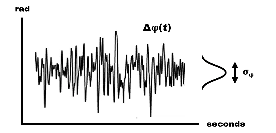
$\Delta f(t)$ = Frequency fluctuations

$\Delta \phi(t)$ = Phase fluctuations

IMPORTANT: Note that here the frequency fluctuations $\Delta f(t)$ are much slower compared to the laser emission frequency $f_0$ , and the amplitude fluctuations $\Delta E(t)$ are much slower compared to the laser emission frequency $f_0$ .

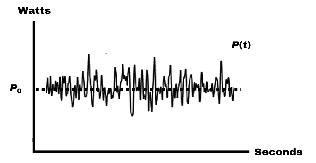
Power/Intensity Fluctuations and Mean Value

Regarding a laser radiation, that is an oscillating electro-magnetic field, a common metric to talk about is Power or even Intensity. The Power, that can be for example measured on a photodetector (composed of a photodiode and a current-to-voltage circuit), is proportional to the squared absolute value of the electric field Amplitude denoted $E(t)=E_0+\Delta E(t)$ , meaning that Power: $P(t) = P_0 + \Delta P(t)$ , where $P_0$ is the mean Power and $\Delta P(t)$ is the Power fluctuations, expressed in Watts (W). Intensity is the optical Power per unit area, so expressed in W/m².

Knowing the laser power and/or intensity is crucial for many applications especially when non-linearity effects are studied or exploited.

For metrology and/or for applications that need as perfect as possible a laser signal, the Power fluctuations is an essential quantity. This Power fluctuations can be analyzed in the time domain to have a simple and first view of it, so a graph with watts over seconds. Then, these power fluctuations could be also reduced by active stabilization, but this is another topic.

Figure 2: Illustration of a laser power fluctuations

P(t)

and the mean value

P_0

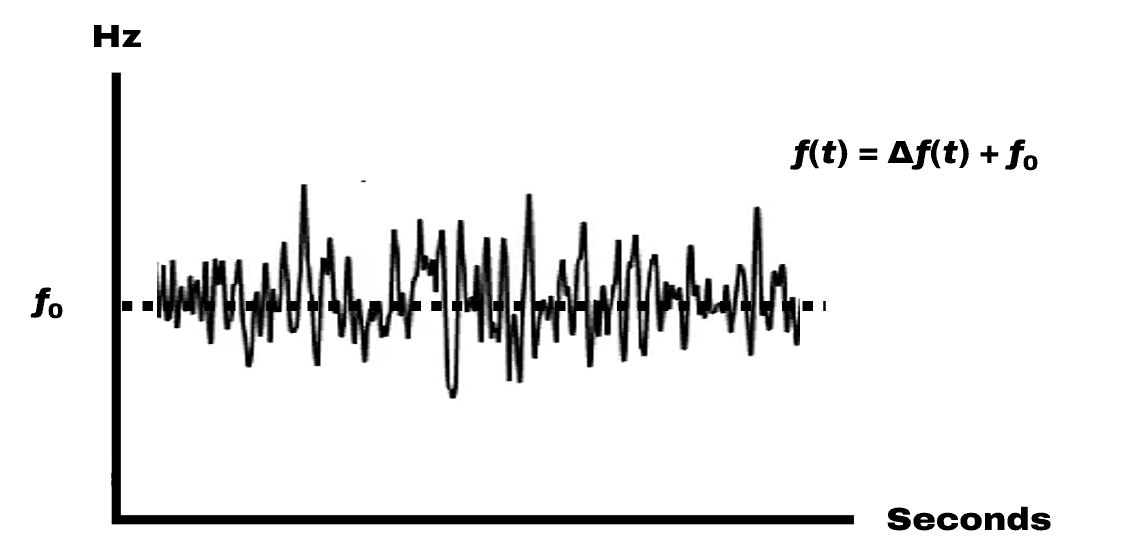
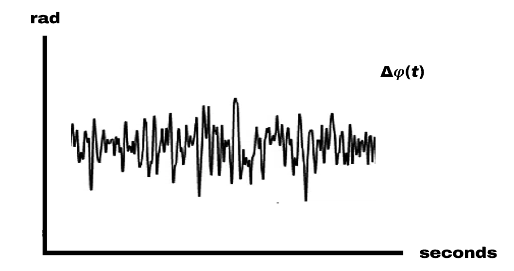
Frequency/Phase Fluctuations and Frequency Mean Value

Frequency and Phase are here in the same section as both gives “similar” information because the frequency is the time derivative of the phase.

Knowing the laser emission frequency and fluctuations is crucial for many applications especially when the laser coherence is concerned and atoms/molecule are involved.

For metrology and/or for applications that need as perfect as possible a laser signal, the frequency/phase fluctuations are essential quantities. These frequency/phase fluctuations can be analyzed in the time domain to have a simple and first view of it, so a graph with Hz or rad over seconds. Then, these frequency phase fluctuations could be also reduced by active stabilization, but this is another topic.

Figure 3: Illustration of a laser frequency fluctuations f(t) and mean value

f_0

Figure 4: Illustration of a laser phase fluctuations

\Delta \phi(t)

FREQUENCY DOMAIN METRICS

In this section, we will present important quantities that can be analyzed in the frequency domain. These quantities are directly what defines the laser emission $\mathbf{E}(t)$ if we restrict it to a simple sine function, as seen in the section above:

$\Delta E(t)$ = Amplitude fluctuations

$\Delta f(t)$ = Frequency fluctuations

$\Delta \phi(t)$ = Phase fluctuations

The time domain view is interesting to see time-dependent events, but it is most of the time difficult to get all the details of a signal from its time domain view. This is why it is common to plot the quantity in the frequency domain, in order to see what the frequencies that compose the signal are and with which contribution/weight.

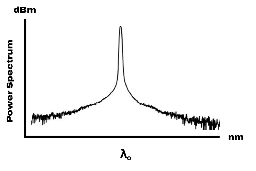
Related to the laser emission, the first quantity that is commonly analyzed into the frequency domain (or even wavelength domain) is the Power emission through the Optical Spectrum measured typically with an Optical Spectrum Analyzer. However, if we consider a single-frequency laser, this frequency view gives mainly a validation of it, gives the mean power, the central frequency ( $f_0$ )/wavelength but not really more, as we are limited by the resolution. Because of this, other methods are needed to get the three quantities of interest here, which are

Frequency Noise
Phase Noise
Relative Intensity Noise

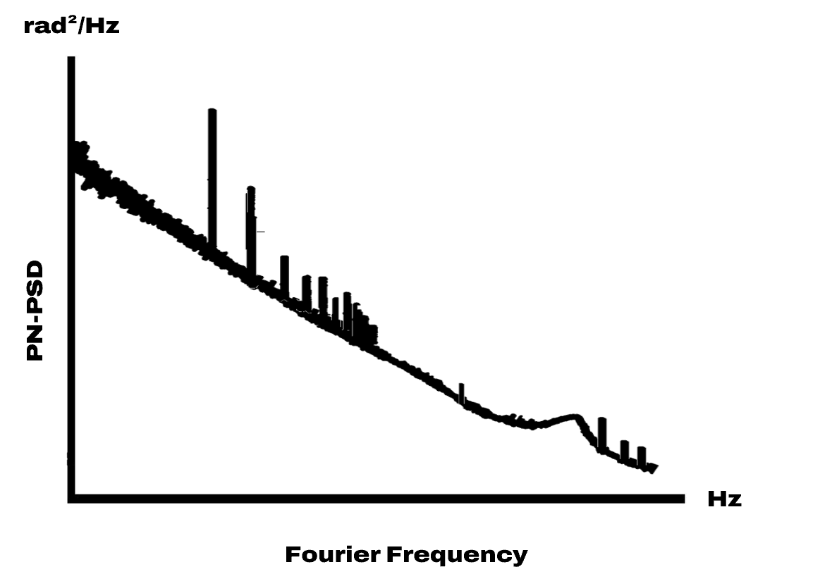
Figure 5: Illustration of a laser Optical Spectrum, showing the power distribution

Phase Noise Power Spectral Density

As defined earlier in this article, knowing the phase fluctuations of a laser is important for different applications. This quantity we wrote it $\Delta \phi(t)$ as a time-dependent function. However, by using the following formula that represents the Fourier Transform of the autocorrelation function of the phase fluctuations, we arrive to a frequency-dependent quantity called Phase Noise Power Spectral Density (PN-PSD):

\begin{equation} S_\phi (f)=\mathcal{F}[R_\phi (\tau)]. \end{equation}

Phase Noise Power Spectral Density is a widely used quantity in the Radio-Frequency community to describe the phase noise of a MHz/GHz electronic oscillator. It has various units like rad²/Hz, rad/sqrt(Hz), and dBc/Hz when we talk about Spectral Purity: $L(f)$ . The Power Spectral Density representation is very important for “energy signal conservation”. This implies that the integration of this signal in the frequency domain remains always the same for any spectral resolution. The PSD view is similar to a classical FFT view with a 1 Hz resolution bandwidth. For an easy reading and to see all the details, it is common that PN-PSD, FN-PSD, and RIN-PSD are in log-log scale.

Figure 6: Illustration of a laser Phase Noise Power Spectral Density

Frequency Noise Power Spectral Density

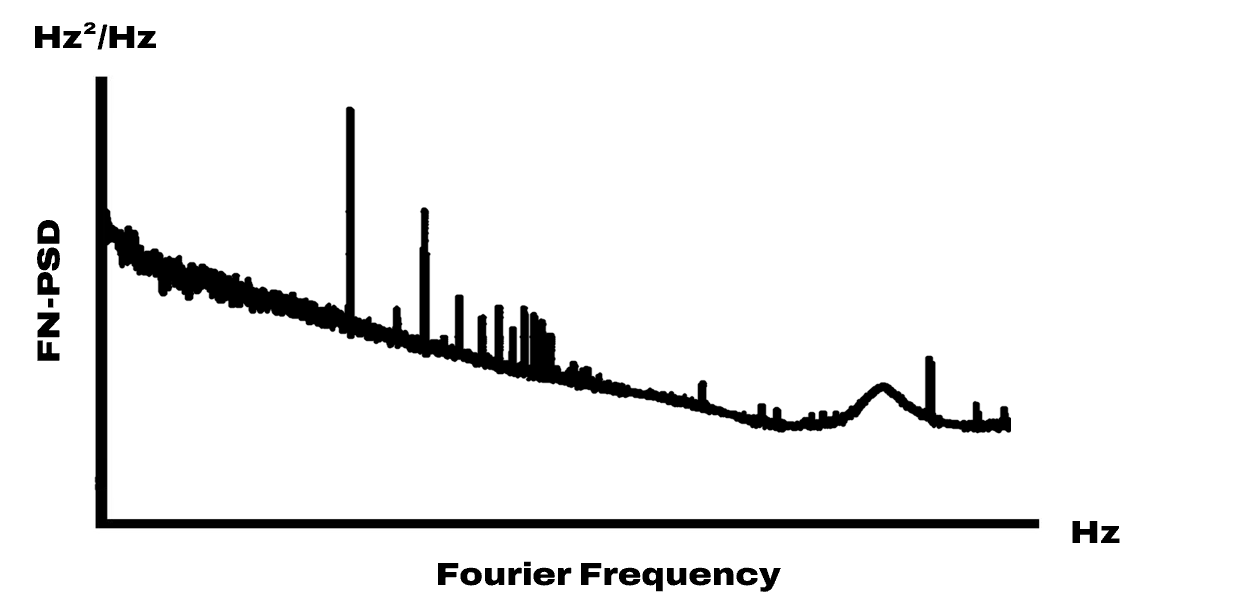
Frequency Noise Power Spectral Density is a frequency-dependent quantity that shows similar information as a PN-PSD. There is a simple and quick relation between the two quantities that is

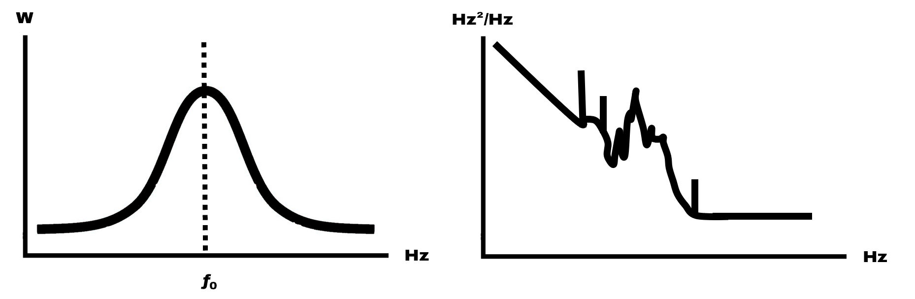
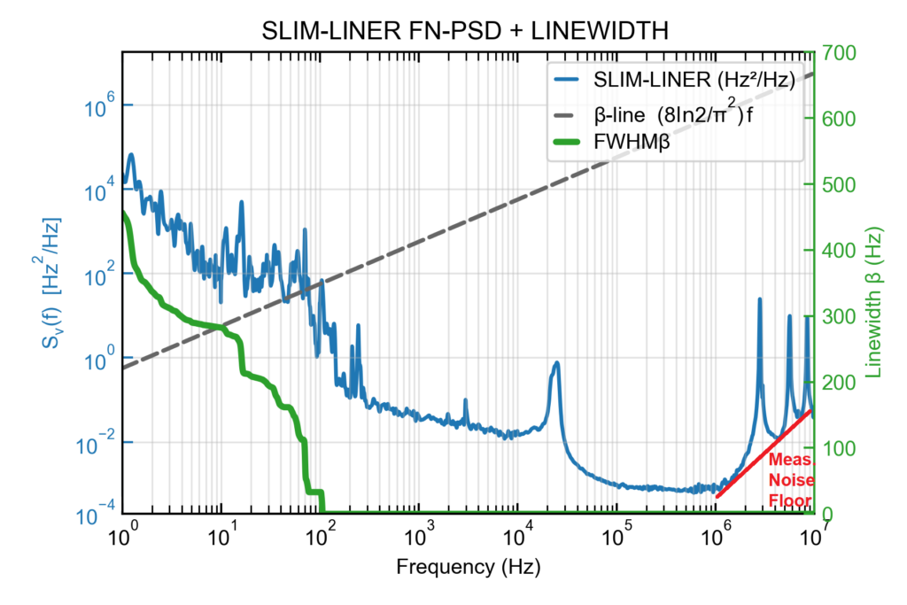
\begin{equation} S_\nu (f)=f^2 \cdot S_\phi (f). \end{equation}

Then, there is a direct and simple noise relation between frequency and phase as shown later in this article. From FN-PSD and PN-PSD, we can see a lot of things to analyze the laser performance, as presented in another article. On the plot below, we can see for example “electronic” noise with thin, high peaks in the middle of the spectrum, “thermal” noise with the increase of the noise when the Fourier frequency is decreasing, and also more “quantum” noise with a white frequency noise floor at high Fourier frequencies that is representative of the “Schawlow-Townes” linewidth. FN-PSD is generally expressed in Hz²/Hz or Hz/sqrt(Hz).

Figure 7: Illustration of a laser Frequency Noise Power Spectral Density

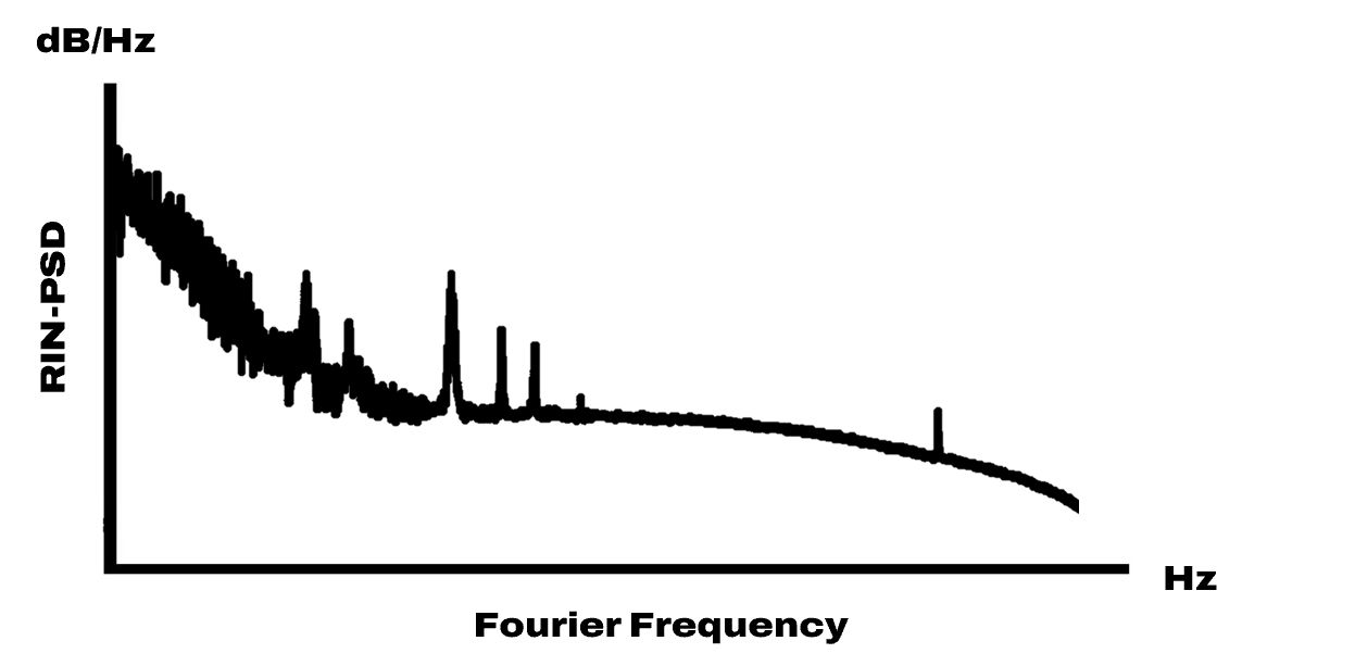
Relative Intensity Noise Power Spectral Density

The last quantity we want to talk about is the Relative Intensity Noise Power Spectral Density, commonly called RIN. This is a frequency view of the laser power fluctuations normalized by the laser mean power. It is calculated, as the PN-PSD and FN-PSD, by the Fourier transform of the autocorrelation function of the power fluctuations normalized first by its mean value:

\begin{equation} \text{RIN} = \mathcal{F}[R_{P/P_0} (\tau)]. \end{equation}

Below is a graph of a typical laser RIN, expressed in dB/Hz, or even sometimes written dBc/Hz, 1/Hz and in dBm/Hz, W/Hz when not normalized to the mean power.

Figure 8: Illustration of a laser Relative Intensity Noise Power Spectral Density

TIME/FREQUENCY INTEGRATION-BASED METRICS

In the previous sections, we have presented the basic/main quantities that define an oscillator emission, such as Power, Phase, and Frequency. From these quantities, that can be analyzed/observed in the time or frequency domains, some mathematical operations are possible to even get more understanding of the oscillator emission. These operations, at least the ones we will look at, always involve an integration function, over a given time scale. They are the following:

Linewidth & Coherence
Frequency / Phase / Power standard deviation
Integrated Frequency / Phase Noise & Timming Jitter
Frequency Stability

We will not talk about the mean value, for example for the power or the frequency wavelength, as we already presented them above.

Linewidth & Coherence

Linewidth: such a simple and widely used quantity useful to compare quickly oscillators, but very often misunderstood and misused as a sales pitch that makes no physical sense!

First of all, the definition of the linewidth is very simple and is the full (or half in some cases) width at half maximum: FWHM. And this is true for any shapes (Gaussian, Lorentzian, Voight…). For a single-frequency laser oscillator, by looking at the power spectrum, it is easy to extract the linewidth (that can also be called −3 dB linewidth instead of FWHM). It means, and this is important, that FWHM is an arbitrary definition and has no real mathematical sense.

In that example, if the linewidth is related to the laser emission, it is in Hz as a unit. Even if getting the linewidth from the power spectrum is easy, getting the laser power spectrum itself is challenging!

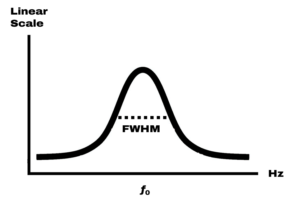
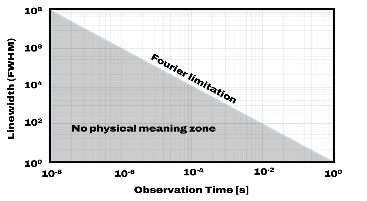
Figure 9: Illustration of a laser linewidth (FWHM) from its Power Spectrum

What is important also to take into account is that the linewidth is an integrated quantity. The linewidth will be different depending on the integration/observation time! This is why giving just a number of a FWHM has no sense, and the integration time should be always given.

So, the easiest way to get the laser linewidth is to beat it against another one that is known as much thinner and that emits a frequency close to it in order to be able to detect it with a fast photodetector. Then, a simple analysis on an Electrical Spectrum Analyzer (ESA) gives the results.

As having another laser at the same wavelength is not always possible, one other possibility is to compute the laser linewidth from its Phase/Frequency Noise PSD. The main challenge here, after being able to measure the laser frequency noise using for example an Optical Frequency Discriminator, is that there is no universal direct mathematical link between FN-PSD and FWHM as, again, FWHM is an “arbitrary” definition.

There is one famous case where there is a direct mathematical link between FN-PSD and FWHM and it is for a laser with pure white frequency noise, so a laser that has a pure Lorentzian shape as its Power Spectrum, and it is given by this formula:

\begin{equation} \text{FWHM} = \pi S_\nu \end{equation}

where $S_\nu$ is the white frequency noise floor in Hz²/Hz. This is commonly called a Lorentzian linewidth, Schawlow Townes linewidth, or even “instantaneous” linewidth as a real laser usually exhibits white frequency noise for Fourier frequencies above 1 MHz.

At SILENTSYS, we call it “commercial” linewidth as it has no physical sense or meaning and this can be confusing and misleading for customers who compare these values for different lasers without having the benefit of hindsight regarding their application’s integration time.

This definition could be fine for lasers that exhibit a very high white frequency noise floor, so a Lorentzian linewidth of let’s say 1–10 MHz, because this noise contribution is probably the dominant one, especially behind “technical noise” that appears mainly at Fourier frequencies below 1 MHz.

IMPORTANT: We advise you to not compare lasers based only on this “instantaneous” linewidth, especially if the value is >> 1 MHz!

To give you more details about why we have this vision at SILENTSYS, that is, from our Time & Frequency background, it has no sense to give a number that is not observable because of the Fourier limitation!
For example, an “instantaneous” linewidth of 1 kHz integrated on 1 µs cannot be measured, because if you look at the power spectrum over 1 µs you will inherently have a resolution limitation of > 1 MHz, as you can see from the graph below!

It is then correct to talk about the FN-PSD, not FWHM!

Figure 10: Illustration of the Fourier Limitation

As there is no direct mathematical link between FN-PSD and linewidth, as for each and real frequency noise spectrum the power spectrum shape is not a pure Lorentzian function, it is still possible to make an estimation, especially based on the so-called beta-separation line method, developed by Di Domenico et al. (2010).

This method simply divides the FN-PSD data into two groups, with values below and above a line, to integrates the parts of the spectrum that contribute to the FWHM. This principle is shown on the next plot where we compute the estimated FWHM of a SLIM LINER laser over different time scales.

*Figure 11: Illustration of the beta-separation line method for FWHM estimation from FN-PSD*

Actually, as demonstrated in the next section, we are working at SILENTSYS on a direct mathematical link to better understand how the linewidth comes from the PN/FN-PSD.

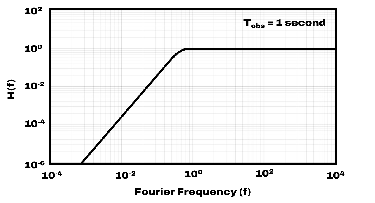
Finally for this section, it is also good to keep in mind that the use of a laser during, for example, 1 ms does not mean that all the Frequency Noise below 1 kHz will not impact the measurement. The observation time does not act as a pure Heaviside filter, but mainly as a second-order high-pass filter with the following formula:

\begin{equation} H(f)=1- \text{sinc}^2(fT_\text{obs}) \end{equation}

\begin{equation} \text{Or even for a Fourier time $(1/f) \gt\gt$ the observation time $T_\text{obs}$}: \quad H(f) \approx \frac{(\pi f T_\text{obs})^2}{3}, \end{equation}

where $f$ is the Fourier frequency and $T_\text{obs}$ is the observation time.

So, even if the laser is observed over 1 ms, all the FN-PSD contributes to its FWHM with less impact for Fourier frequencies below the observation time, which is very important to keep in mind.

Figure 12: Illustration of the Transfer function

H(f)

Coherence: Instead of linewidth, people usually use “Coherence” as a tool to characterize and compare lasers. It can be Coherence time or Coherence length when related to the propagation speed of the wave. Basically, the Coherence time for an oscillator is the duration for which the correlation between the electrical field and itself at these two different times is equal to $e^{-1}$ :

\begin{equation} g(\tau)=\frac{\langle E^*(t) E(t+\tau)\rangle}{\sqrt{\langle |E(t)|^2 \rangle \langle |E(t+\tau)|^2\rangle}} \quad |g(\tau)| \in [0,1] \quad |g(\tau_c)|=e^{-1}. \end{equation}

So, in reality, contrary to what is commonly assumed, even if we interfere a laser with itself at two time instances that are a way larger than the coherence time, we will still see interference fringes. However, this is possible by looking at the signal very fast, so during a very short time scale. If we now look at the interferences during a long time (so to integrate the signal), we will not see fringes anymore but just a constant value.

In conclusion, the coherence time of a laser is directly related to the Phase/Frequency noise of the laser as we will see later in this article.

Frequency/Phase/Power Standard Deviation

In our case, looking back at the timeseries of the oscillator Phase and Frequency fluctuations, one interesting statistical parameter here is the standard deviation. The standard deviation ( $\sigma_x$ ) is a common statistical parameter that we will not develop here. However, one important relation between the Phase Frequency standard deviation and the Phase/Frequency noise power spectral density is that we can compute this quantity by integrating the spectrum and taking the root mean square as shown in the next formula. It is true because of few statistical considerations on the Phase/Frequency fluctuation distribution. This is also what we call Integrated Phase/Frequency noise. It is possible to do the same also for the Power and for the Timing Jitter.

Figure 13: Illustration of the standard deviation of a laser phase fluctuations

\Delta \phi(t)

\begin{equation} \sigma^2_\phi=\int\limits_{-\infty}^\infty S_\phi (f) df \quad \text{and} \quad \sigma^2_f=\int\limits_{-\infty}^\infty S_f (f) df \end{equation}

Integrated Frequency/Phase Noise & Timing Jitter

As shown in the previous section, from the Frequency/Phase noise spectrum, we can make an integration to reach the so-called Integrated Frequency Noise (in Hz) and the Integrated Phase Noise (in rad). These quantities are often used in the Time and Frequency metrology community. They also are used to compare different oscillators/lasers. However, it is also very important to give the Integration Range when giving a value. These quantities are also related to laser linewidth and coherence. Instead of giving only one value, it is common to show the integration over the Fourier frequencies in order to give more details on the noise contributions.

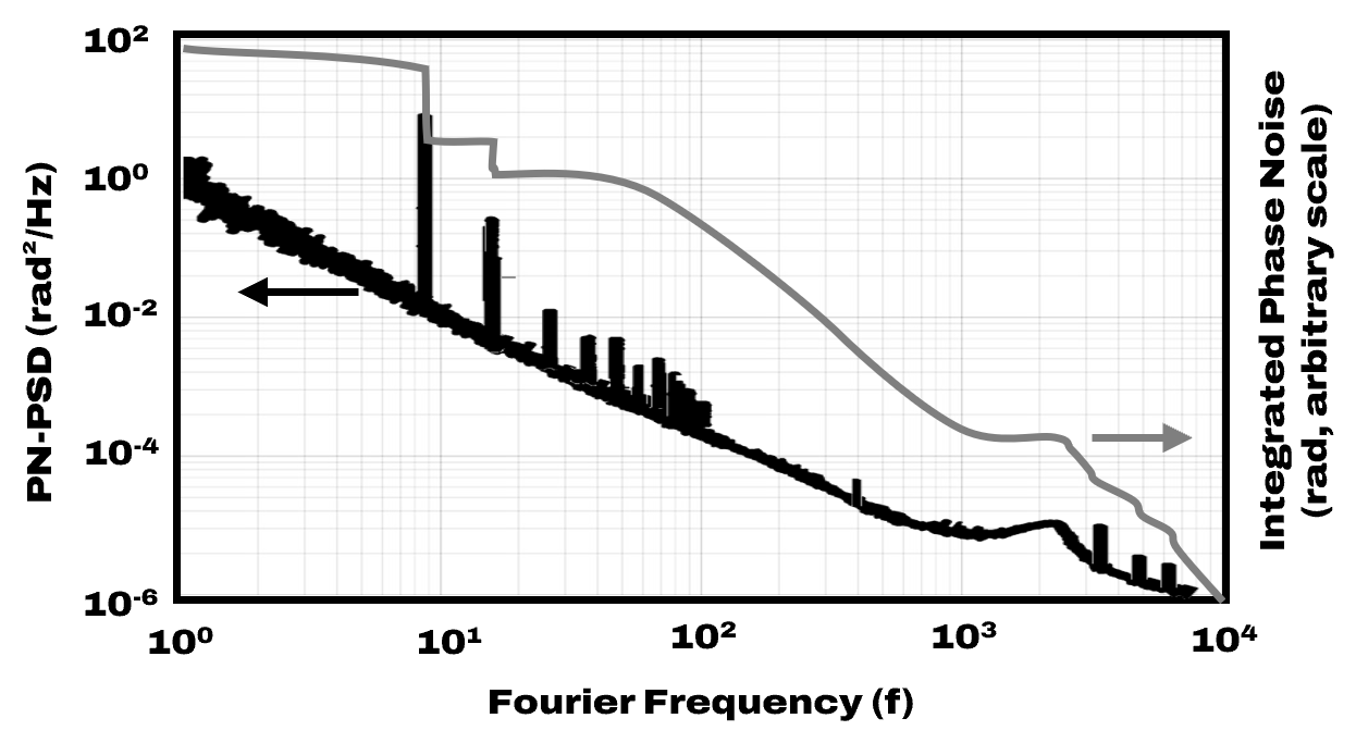
Figure 14: Illustration of Integrated Phase Noise

Instead of Integrated Phase noise, another quantity is commonly used: the Timing Jitter, in seconds. Simply, it is another view compared to the phase noise by normalizing to the carrier frequency of the signal in order to talk about time and not phase.

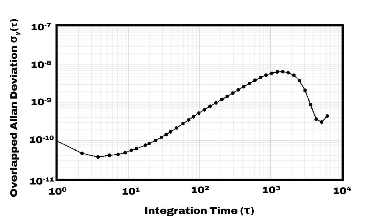
\begin{equation} \phi_\text{rms}=\sqrt{\int\limits_{f_\text{min}}^{f_\text{max}} S_\phi (f) df} \qquad \nu_\text{rms}=\sqrt{\int\limits_{f_\text{min}}^{f_\text{max}} S_\nu (f) df} \qquad t_\text{rms}=\frac{\phi_\text{rms}}{2\pi f_0} \end{equation}

Frequency Stability

Now, when we study the frequency “drift” or “long-term” frequency fluctuations of an oscillator, other tools have been developed by the Time and Frequency metrology community. Indeed, the frequency noise PSD introduced in the previous section is a powerful tool to characterize the frequency fluctuations of an oscillator over short time scales (typically shorter than 1 s, corresponding to Fourier frequencies above 1 Hz). The frequency fluctuations over longer time scales (Fourier frequencies typically below 1 Hz) are generally characterized differently, from the time series of the oscillator frequency $\nu$ recorded with a frequency counter. This time series is generally normalized to the averaged oscillator frequency $\nu_0$ , $y=\nu/\nu_0$ , to reach relative fluctuations in order to compare easily oscillators (clocks) at different carrier frequencies. The frequency stability of the oscillator is characterized by the so-called Allan variance (AVAR), which describes how well the oscillator reproduces the same frequency over a given time $\tau$ :

\begin{equation} \sigma^2_y(\tau)=\frac{1}{2(N-1)}\sum_{i=1}^{N-1}(\bar{y}_{i+1} – \bar{y}_i)^2, \end{equation}

where $N$ is the number of frequency samples averaged during the integration time $\tau$ . The Allan variance $\sigma^2_y(\tau)$ or the Allan deviation $\sigma_y(\tau)$ are unitless and represent the relative frequency stability of the oscillator. Other definitions exist in order to better analyze the frequency fluctuations, for example, HVAR, PVAR, MVAR, TVAR….

*Figure 15: Illustration of Overlapped Allan Deviation*

LINK BETWEEN METRICS (COMING SOON)

Did you enjoy this article? Would you like to contribute or give your opinion? Contact us.