Narrow-linewidth and frequency-stable lasers are nowadays key components in reaching high performances in many domains and applications where the laser interferometry process is involved, like for LiDAR, SENSING, METROLOGY, QUANTUM TECHNOLOGIES, …. Making a narrow-linewidth laser that is compact, low cost, and can handle hard environment (temperature, acoustics, vibrations…) is very challenging but not impossible. The key point to succeed in it is to better understand first the physical metrics behind it (linewidth, frequency and phase noise, frequency stability…) and the technological methods to improve a laser in order to get a much more coherent one.
As we describe in another article, a laser does not exhibit a “pure” emission frequency. The laser emission frequency is not an ideal sine wave in the time domain and not a delta Dirac function in the frequency domain. The laser emission frequency fluctuates over time, with different amplitudes at different time scales, which gives it a linewidth and a given frequency stability.
The best way to characterize and stabilize the laser is by being able to detect the laser frequency fluctuations, which is done with an OPTICAL FREQUENCY DISCRIMINATION scheme.
OPTICAL FREQUENCY DISCRIMINATION: DEFINITIONS
OPTICAL FREQUENCY DISCRIMINATION, or LASER FREQUENCY DISCRIMINATION, is a technique that gives the frequency evolution in the time domain of a single-frequency under-test laser. So, these are methods that convert laser frequency emission into a readable signal, because, in contrast to electronic oscillators, a laser emits an electric field at very a high frequency, typically around 200 THz for telecom lasers (1.5 µm wavelength). Different techniques have been developed during the past, with pros and cons for each of them. We can classify OPTICAL FREQUENCY DISCRIMINATION techniques into two main categories: ABSOLUTE and RELATIVE.
RELATIVE OPTICAL FREQUENCY DISCRIMINATION gives in real-time the information of the laser frequency fluctuations but without being capable of giving the carrier laser frequency.
ABSOLUTE OPTICAL FREQUENCY DISCRIMINATION can return both the laser frequency fluctuations and the carrier laser frequency.
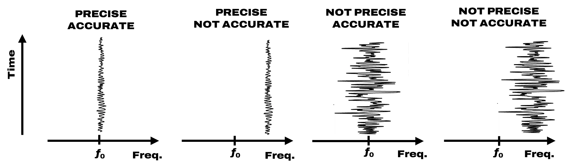
These two different techniques are preferred for specific applications. Having the RELATIVE method can lead to PRECISE measurements while the ABSOLUTE method can lead to PRECISE and ACCURATE measurements.
OPTICAL FREQUENCY DISCRIMINATION: EXAMPLE TECHNIQUES
We present here a non-exhaustive list of OPTICAL FREQUENCY DISCRIMINATION techniques. For all these techniques, we compare the main specifications, which are the following: Optical Bandwidth (working wavelength range), Acquisition Bandwidth (the maximum measurement rate of the laser frequency fluctuations), Size, and Cost. Almost all these techniques are based on optical interferometry. These comparisons are made by us and are by no means a universal truth.
 Diffraction Grating (Optical Spectrum Analyzer)
This technique is based on a spectrograph, which means that the under-test laser is sent to a diffraction grating that will spatially disperse the light which is then going to an array of photodetectors. Therefore, the laser frequency is converted into a spatial position measured by the photodetectors; so by knowing the diffraction grating properties and the geometrical dimensions of the system, it is possible to measure the laser emission frequency. This technique is also compatible with a non–single frequency laser, like a Fabry–Pérot diode laser, Optical Frequency Combs, …. With it, it is possible to reach good accuracy but not good precision.

Fizeau Interferometer (Wavemeter)
This technique consists of a Fizeau-based interferometer that generates an interference pattern, directly linked to the under-test laser frequency, on an array of photodetectors. The measured electrical signal can then be used to retrieve the laser frequency. With this technique, it is possible to reach very good accuracy and good precision.

Heterodyne Detection (Reference Laser)
This technique consists of combining the laser under test with an external laser source (that is considered as the reference) and to send them into a fast photodiode. The photodiode will generate a signal (beat note) that is the frequency difference of the two lasers, so it converts the laser under test from the optical domain to the electrical domain in order to be then evaluated, with for example an Electrical Spectrum Analyzer or a Frequency Counter. This represents a very simple technique. However, the reference laser must be better than the under-test laser (in terms of frequency fluctuations) to be sure that the radio-frequency signal obtained is mainly representative of it. This also limits drastically the optical bandwidth accessible as the reference laser should be not more distant than few tens of GHz from the laser under test to be able to easily detect the beat note and to analyze it. The level of accuracy and precision of this technique will mainly depend on the reference laser. This reference laser can be a free-running laser, a stabilized laser (to an atomic reference for example), an optical frequency comb….
An optical frequency comb referenced to an atomic clock with fast electronics is probably the highest performance OPTICAL FREQUENCY DISCRIMINATOR, but with tremendous cost.

Spectroscopy (Atomic or Molecular Absorption/Transition)
This technique is the only one in our list that is not based on an interferometric process of light. It uses the interaction between light and matter, and especially the properties of light, to absorb differently depending on the light wavelength/frequency. This technique is considered the most accurate one, depending on the atom used.

Optical Cavity (Multiple-Wave Interferometer)
This technique consists of interfering the input laser with itself a lot of times in order to create interference fringes, so laser frequency values where the light is quasi-totally transmitted (constructive interferences) and values where the light is quasi-totally reflected (destructive interferences). As the fringes have a Lorentzian shape, where the fringe width depends on the Quality Factor (Q) and the fringe-to-fringe distance depends on the cavity length (FSR: Free Spectral Range), the transmitted or reflected optical power will be directly linked to the input laser frequency. Many types of optical cavities exist, like all fibered-based ring cavity or free-space Fabry–Pérot (FP) cavity. Each of them has pros and cons, and the most performant one is the “Ultra-Stable Cavity” based on a FP architecture with very high reflective mirror coatings, placed under vacuum and with ULE (Ultralow Expansion) design to make the optical length changes with temperature as low as possible. This technique probably offers the most precise and fast optical frequency discrimination, but it is highly constrained by its size and cost and does not provide accuracy.

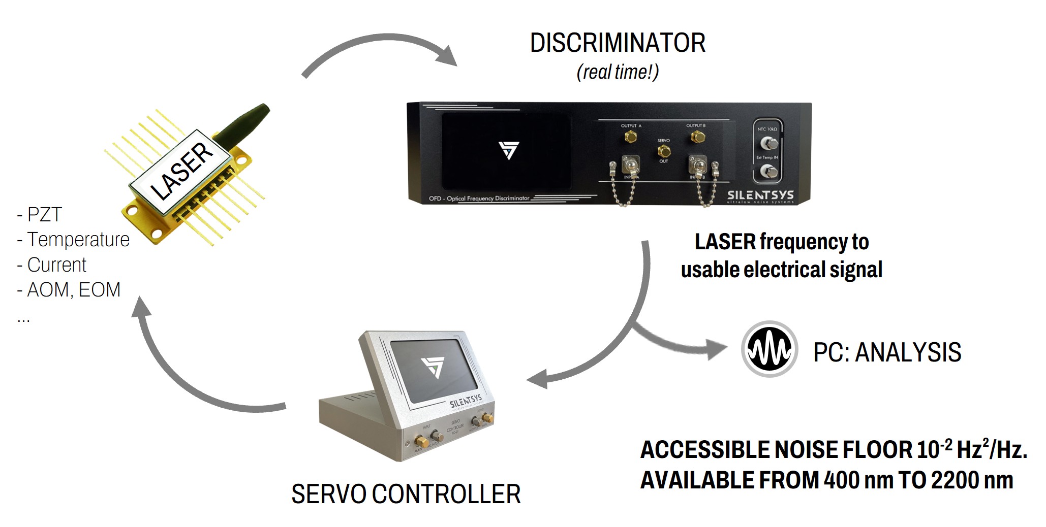
OPTICAL FREQUENCY DISCRIMINATION: from SILENTSYS
At SILENTSYS, we are also doing OPTICAL FREQUENCY DISCRIMINATION, that is directly integrated in a few of our products like the OFD (Optical Frequency Discriminator) or the OFC (Optical Frequency Correlator). We provide OPTICAL FREQUENCY DISCRIMINATION that is small, fast, affordable, and available from 400 nm to 2200 nm with a typical working range of 100 nm around the central wavelength.
These are based on modified Michelson or Mach–Zehnder fiber interferometers, with a high vibrations/acoustics isolation and high-level temperature stabilization (at the microkelvin level) and ultralow noise photodetection in order to reach very good laser frequency discrimination precision. However, we do not provide accuracy at the moment. More details on the use of the OFD and OFC are presented in other articles.

HOW DOES IT WORK?
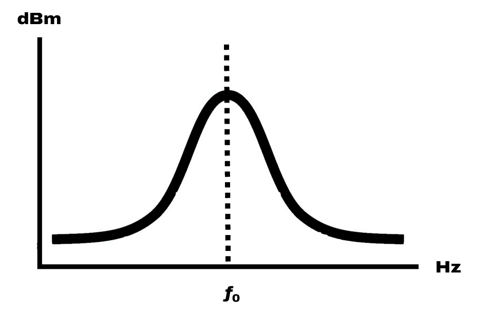
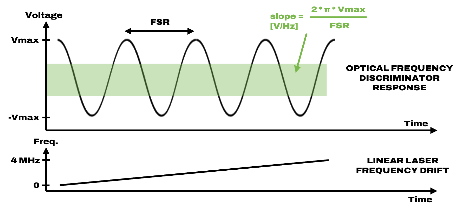
As the SILENTSYS OFD/OFC are based on modified Michelson or Mach–Zehnder interferometers, so a 2-wave interferometric process, the result is a sine fringes pattern against the change of the input laser frequency. At the middle of one fringe (the green zone on the Figure 3), the conversion between laser frequency fluctuations and output voltage is linear, so it is then possible to retrieve the laser frequency fluctuations by recording the voltage time trace of the OFD and by knowing 2 important parameters, which are the amplitude of the fringes (Vmax) and the OFD free spectral range (so the frequency distance between 2 fringes).
In the next figure, as the laser is going through 4 fringes by changing its frequency of 4 MHz, this means that the FSR is 1 MHz in this specific case. The OFD FSR is fixed by construction and can be adjusted at the order between 2 MHz and 2 GHz (other values possible on demand).
These products make good candidates for laser frequency stabilization or characterization, enabling Frequency Noise PSD measurement, Frequency Stability analysis, and Frequency Noise reduction by more than 60 dB to reach a Hz-level laser linewidth from a MHz one. The frequency stabilization is very easy as there is no need for an external laser frequency modulator, complex locking schemes (such as Pound–Drever–Hall), and cavity scanning as with the OFD/OFC there is a locking point each half of FSR, for example, each 5 MHz (FSR of 10 MHz) compared to each 1 GHz with a 15 cm long FP cavity.